Cluster Detection in PCoA Space using Kernel Density Estimation

Two Group Comparison

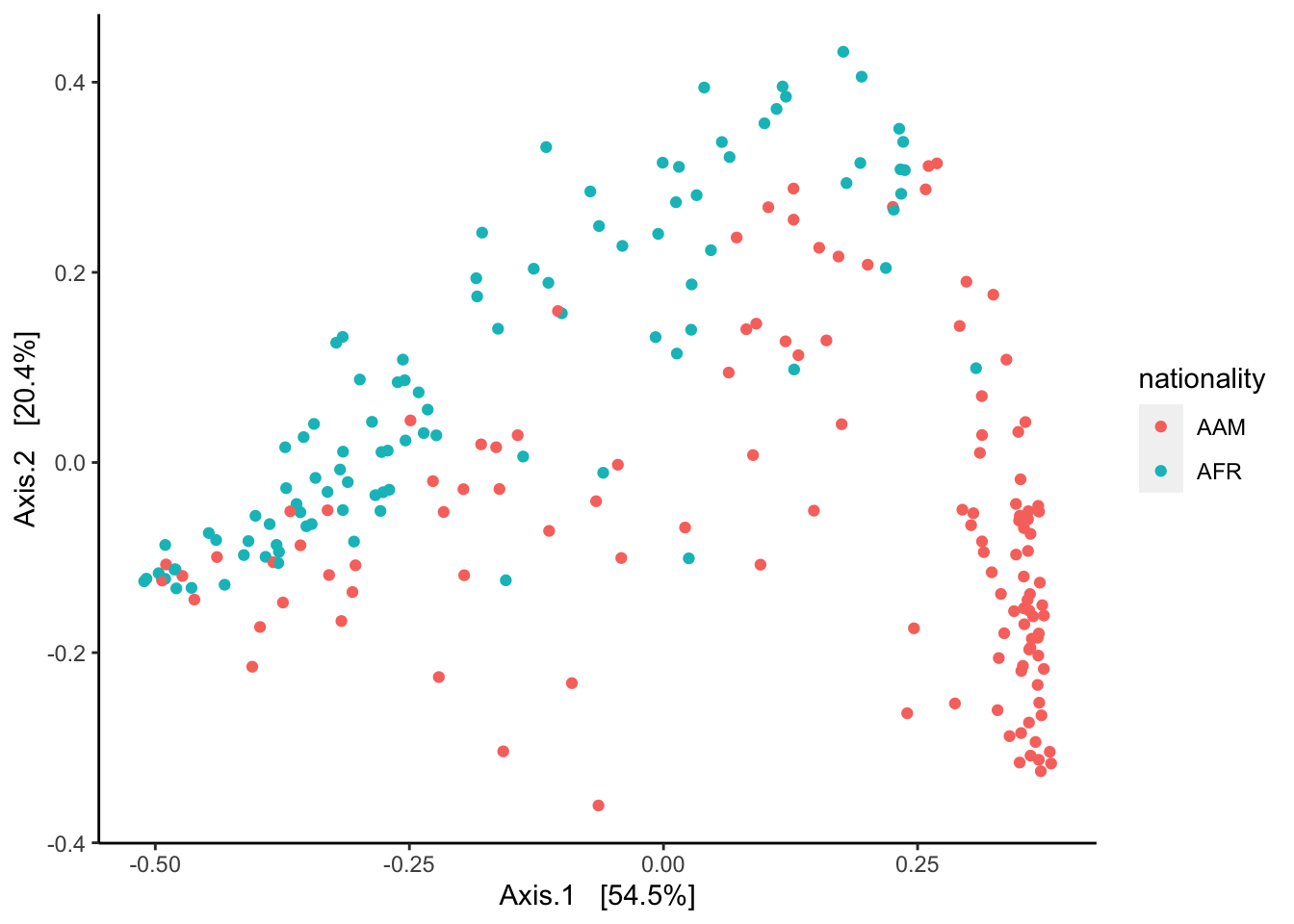
As an example of relative spatial clustering between two groups I compare the two levels of the nationality variable “AMR” (America) and “AFR” (Africa). A plot of the samples by the two groups is displayed below:

# Plot ordination
phyloseq::plot_ordination(pseq.core, ord, color = "nationality") +
  ggplot2::geom_point(size = 1) + 
  ggplot2::theme(panel.grid.major = ggplot2::element_blank(),
                 panel.grid.minor = ggplot2::element_blank(),
                 panel.background = ggplot2::element_blank(),
                 axis.line = ggplot2::element_line(colour = "black"))

To detect significant relative spatial clustering between the two nationalities, I use the risk function from the sparr package. The function requires data as a planar point process (ppp) object. Here, I use the default settings for the risk function except I use adaptive-bandwidth selection. Significant areas are defined as areas that exceed a two-tailed 0.05 alpha level.

# Convert to ppp object
test_df <- data.frame("x" = ord$vectors[,1],
                      "y" = ord$vectors[,2],
                      "g" = pseq@sam_data@.Data[[3]])
sp::coordinates(test_df) <- ~ x + y
test_pp <- as(test_df, "ppp")

# Spatial Relative Risk Function
f0 <- sparr::risk(test_pp, tolerate = TRUE, adapt = TRUE)

# Plot of significant areas
f0_p <- f0$P
f0_p$v <- factor(ifelse(f0_p$v < 0.025, "AAM",
                        ifelse(f0_p$v > 0.975, "AFR","insignificant")),
                 levels = c("AFR", "insignificant", "AAM"))
spatstat.geom::plot.ppp(test_pp, ann = TRUE, axes = TRUE,
                        leg.side = "left",
                        xlab = "Axis.1 [54.5%]",
                        ylab = "Axis.2 [20.4%]",
                        main = "Significant area, adaptive bandwidth, alpha = 0.05",
                        cols = c("coral1", "cadetblue3"),
                        pch = 16)
spatstat.geom::plot.im(f0_p, add = TRUE, show.all = TRUE, main = "",
                       col = c("cadetblue4","grey80","coral4"))
spatstat.geom::plot.ppp(test_pp, add = TRUE, main = "",
                        cols = c("coral1", "cadetblue3"),
                        pch = 16)

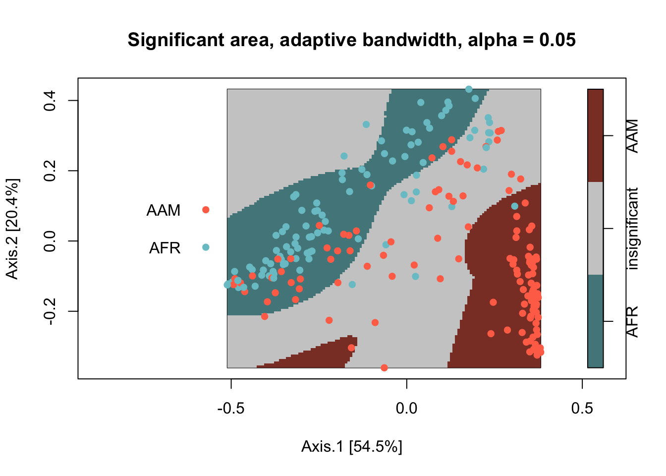
The African group has one significant cluster relative to the American Group (colored blue), which has two significant clusters (colored red). The areas in grey are where the African and American groups spatially covary together that is indiscernible from spatial randomness.

Multi-Group Comparison

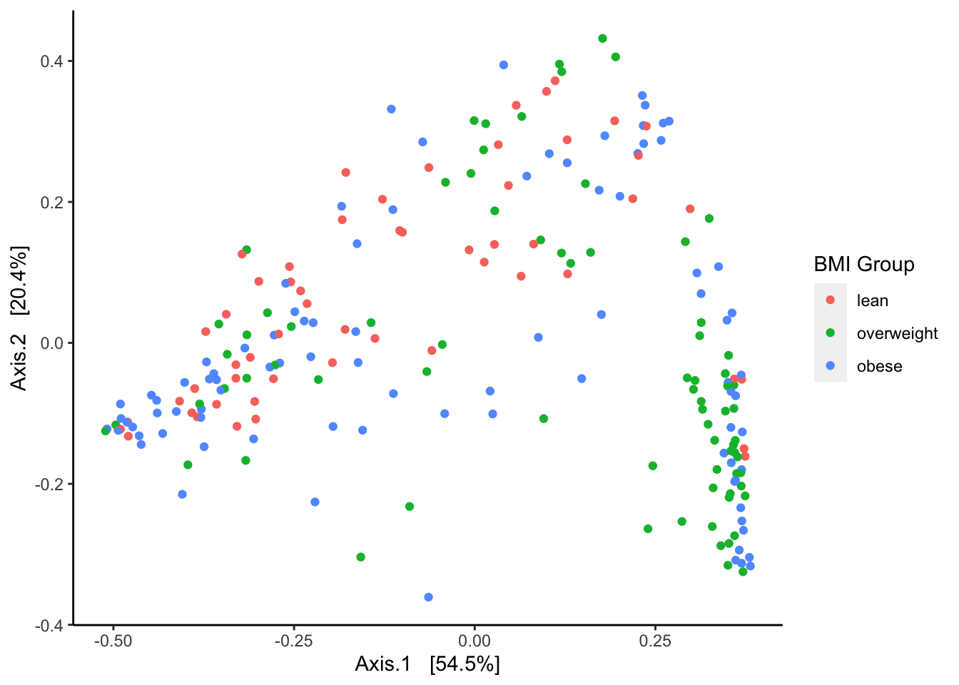
As an example of relative spatial clustering between three groups I compare the two levels of the bmi_group variable “lean”, “overweight’ and”obese”. A plot of the samples by the three groups is displayed below:

# Plot ordination
phyloseq::plot_ordination(pseq.core, ord, color = "bmi_group") +
  ggplot2::geom_point(size = 1) +
  ggplot2::labs(color = "BMI Group") +
  ggplot2::theme(panel.grid.major = ggplot2::element_blank(),
        panel.grid.minor = ggplot2::element_blank(),
        panel.background = ggplot2::element_blank(),
        axis.line = ggplot2::element_line(colour = "black"))

To detect significant relative spatial clustering between three BMI groups, I use a spatial segregation model relrisk from the spatstat package. The function requires data as a planar point process (ppp) object. Here, I use the default settings for the relrisk function. I present 1) the most common BMI group across the MDS/PCoA space, and 2) areas that are significantly different from the null expectation for each BMI group. See my previous post about using the spatial segregation model.

# Convert to ppp object
test_df <- data.frame("x" = ord$vectors[,1],
                      "y" = ord$vectors[,2],
                      "g" = pseq@sam_data@.Data[[8]])
sp::coordinates(test_df) <- ~ x + y
test_pp <- as(test_df, "ppp")

# Spatial Segregation model
f1 <- spatstat.core::relrisk.ppp(test_pp, se = T)

# Plot of most common BMI Group
wh <- spatstat.geom::im.apply(f1$estimate, which.max)
types <- levels(spatstat.geom::marks(test_pp))
wh <- spatstat.geom::eval.im(types[wh]) # most common 

spatstat.geom::plot.ppp(test_pp, ann = TRUE, axes = TRUE,
                        leg.side = "left",
                        xlab = "Axis.1 [54.5%]",
                        ylab = "Axis.2 [20.4%]",
                        main = "Most common type",
                        cols = c("coral1", "chartreuse3", "cadetblue3"),
                        pch = 16)
spatstat.geom::plot.im(wh, add = TRUE, show.all = TRUE, main = "",
                       col = c("coral4","cadetblue4","chartreuse4"))
spatstat.geom::plot.ppp(test_pp, add = TRUE, main = "",
                        cols = c("coral1", "chartreuse3", "cadetblue3"),
                        pch = 16)

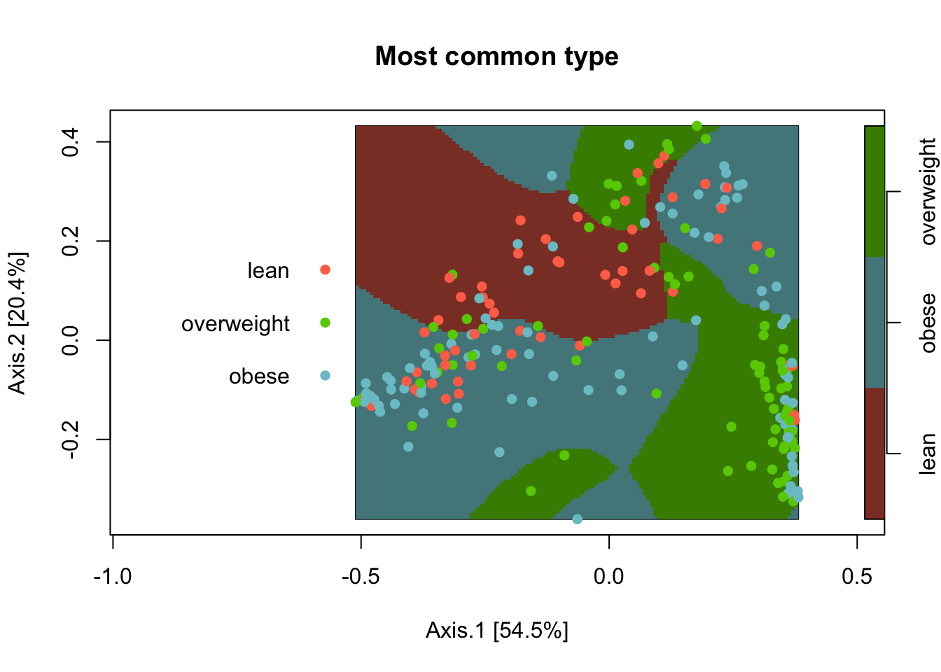
The “lean” BMI group appears most common in one area of the MDS/PCoA space (colored red), while the other two groups have numerous clusters. This plot does not indicate where eat group are significantly different from their null expectations. For example, our null expectation for the “lean” BMI group is a probability of about 0.25 (56/222).

#spatstat::plot.im(wh, main="Most common type", ribargs = list(las = 1))

# Plot of significantly different areas
alpha <- 0.05                           # alpha
z <- qnorm(alpha/2, lower.tail = F)     # z-statistic
f1$u <- f1$estimate + z*f1$SE           # Upper CIs
f1$l <- f1$estimate - z*f1$SE           # Lower CIs
mu_0 <- as.vector(table(spatstat.geom::marks(test_pp))/test_pp$n) # null expectations by type
f1$p <- f1$estimate # copy structure of pixels, replace values
for (i in 1:length(f1$p)) {
  f1$p[[i]]$v <- factor(ifelse(mu_0[i] > f1$u[[i]]$v, "lower",
                               ifelse( mu_0[i] < f1$l[[i]]$v, "higher", "none")),
                        levels = c("lower", "none", "higher"))
}

# Plot significant p-values
plot(f1$p, main = "Significant difference from null?")

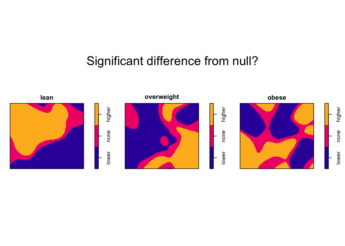
The “lean” BMI group is significantly higher than expected in one large cluster. The “overweight” BMI group is significantly higher than expected in one large cluster and one small cluster. The “obese” BMI group is significantly higher in numerous small clusters.