Areas of a spatial segregation model significantly different from null expectations
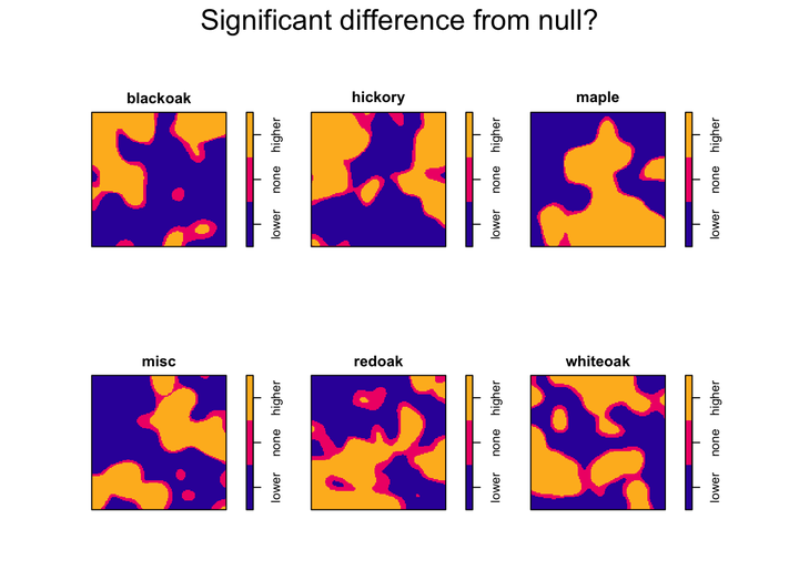 Image credit:
Ian Buller
Image credit:
Ian Buller
I present code to identify areas of a spatial segregation model that exceed our null expectations using the relrisk function in the spatstat package and an assumption of normality of the estimated probabilities.
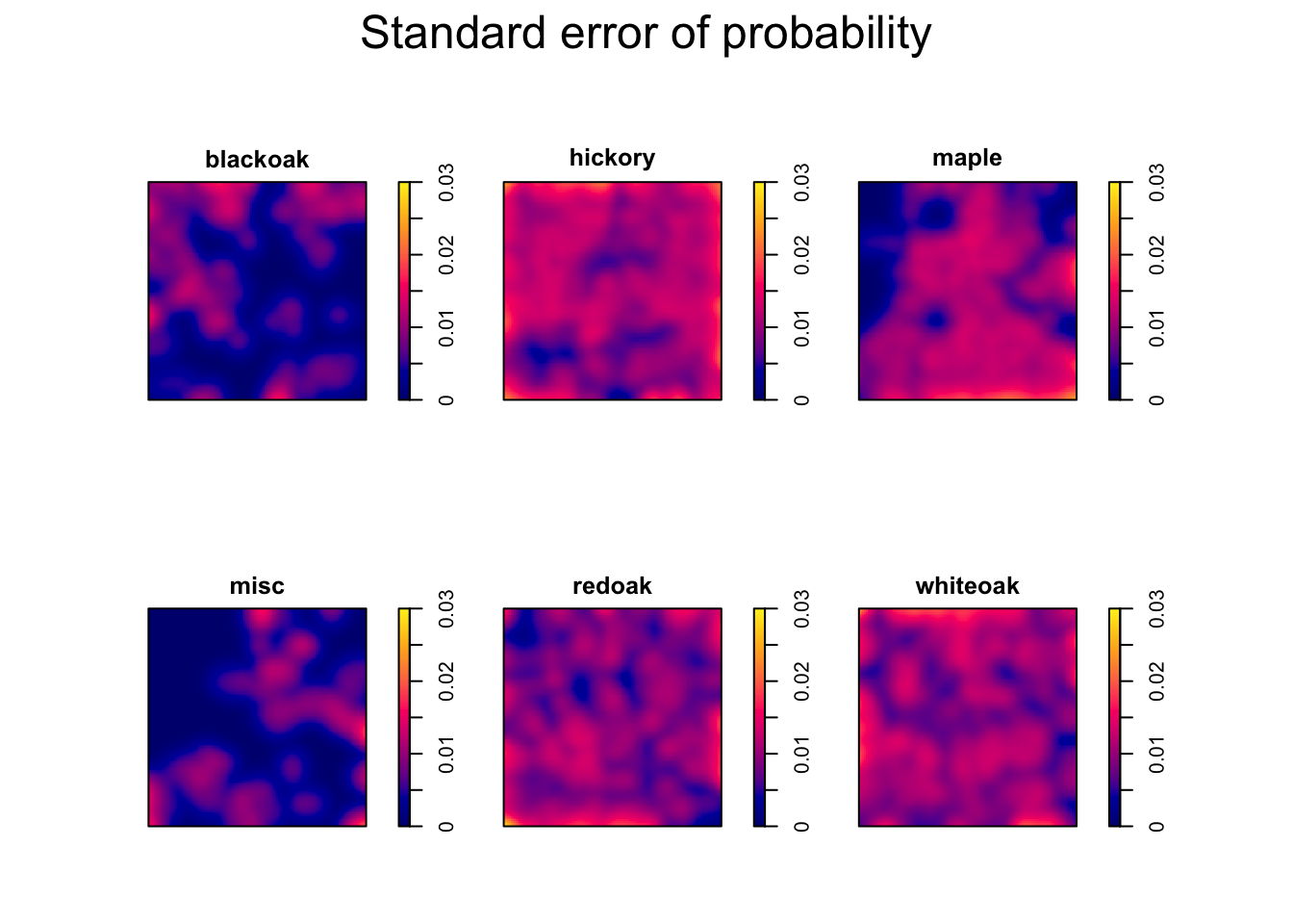
A spatial segregation model was originally proposed by Diggle, Zheng, & Durr in 2005 which estimates spatially-varying probabilities of an event of a certain type to occur in an area accounting for other types. The original method uses a Monte Carlo-based simulation, which is computationally expensive. Instead, Adrian Baddeley and the spatstat team adapted the relrisk function for a multitype (m > 2) point pattern that has an option to compute the standard error of the probability estimates based on asymptotic theory, assuming a Poisson process.
Here, I use the standard errors to compute a 95% confidence interval (CI) at all gridded pixels (“knots”) for each type. Knots with a CI that does not capture the null expectation for each type are identified. I use the provided lansing dataset from the
spatstat.data package. Created with assistance from
Dr. Lance Waller and
Barry Rowlingson.
# Packages
loadedPackages <- c("spatstat")
invisible(lapply(loadedPackages, require, character.only = T))
# Data
  lansing
## Marked planar point pattern: 2251 points
## Multitype, with levels = blackoak, hickory, maple, misc, redoak, whiteoak
## window: rectangle = [0, 1] x [0, 1] units (one unit = 924 feet)
# Convert the lansing data to a ppp object
  ppp_lansing <- ppp(
    x = lansing$x,
    y = lansing$y,
    window = unit.square(),
    marks = as.factor(marks(lansing))
  )

# Plot input
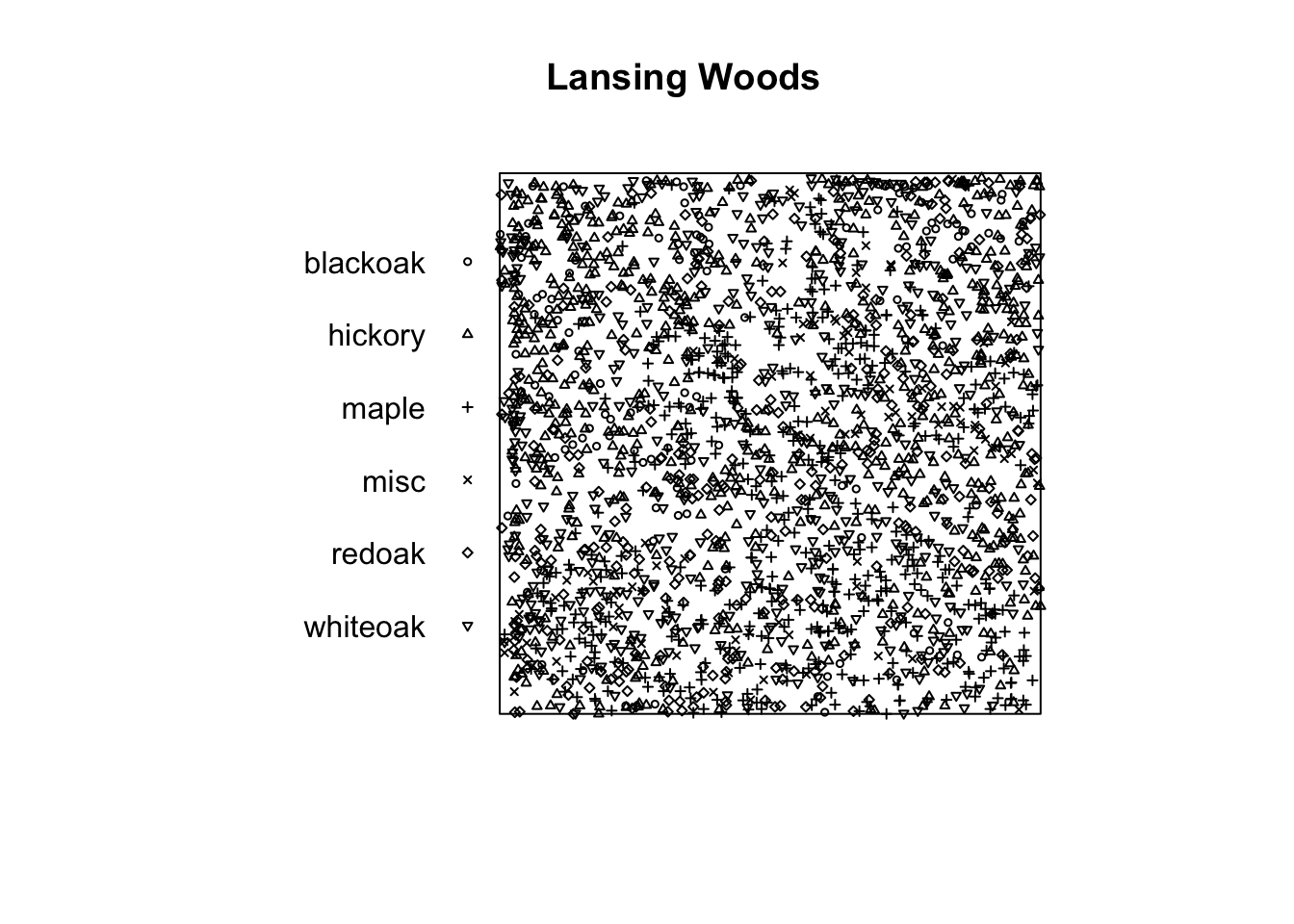
  plot.ppp(ppp_lansing, main = "Lansing Woods", cex = 0.5)
# Estimate nonparametric spatially-varying probabilities of type
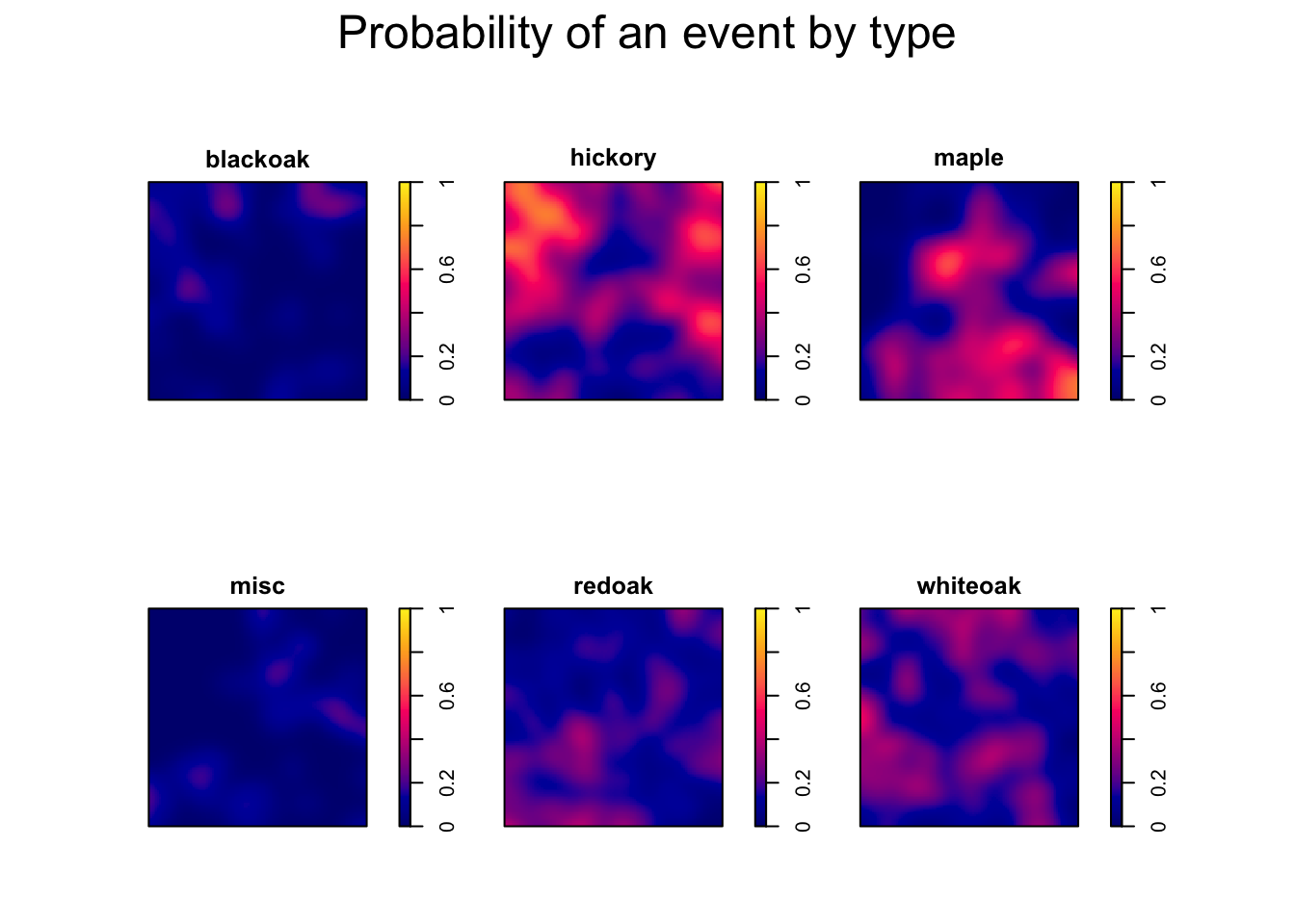
  f1 <- relrisk.ppp(ppp_lansing, casecontrol = F, diggle = T, se = T, sigma = bw.diggle)

# Default plots
  plot(f1$estimate, main = "Probability of an event by type", zlim = c(0,1)) # probabilities
plot(f1$SE, main = "Standard error of probability", zlim = c(0,0.03)) # standard errors
  wh <- im.apply(f1$estimate, which.max)
  types <- levels(marks(lansing))
  wh <- eval.im(types[wh]) # most common
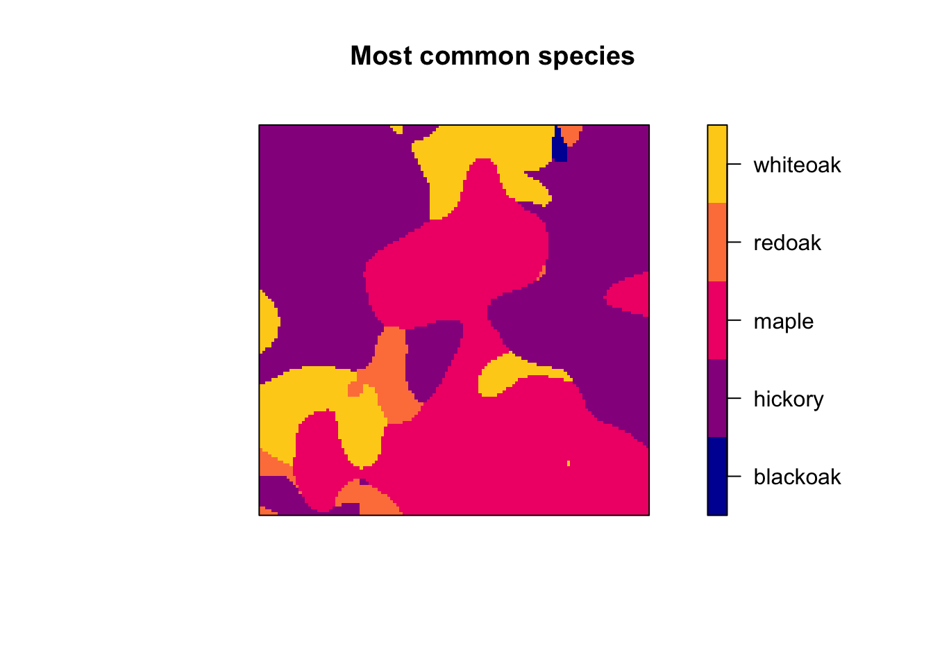
  plot.im(wh, main="Most common species", ribargs = list(las = 1))
# Significant p-values assuming normality of the Poisson process
## relrisk() computes standard errors based on asymptotic theory, assuming a Poisson process
  alpha <- 0.05                           # alpha
  z <- qnorm(alpha/2, lower.tail = F)     # z-statistic
  f1$u <- f1$estimate + z*f1$SE           # Upper CIs
  f1$l <- f1$estimate - z*f1$SE           # Lower CIs
  mu_0 <- as.vector(table(marks(ppp_lansing))/ppp_lansing$n) # null expectations by type
  f1$p <- f1$estimate # copy structure of pixels, replace values
  for (i in 1:length(f1$p)) {
    f1$p[[i]]$v <- factor(
      ifelse(
        mu_0[i] > f1$u[[i]]$v, "lower",
             ifelse(mu_0[i] < f1$l[[i]]$v, "higher", "none")
      ),
      levels = c("lower", "none", "higher"))
  }

  # Plot significant p-values
  plot(f1$p, main = "Significant difference from null?")
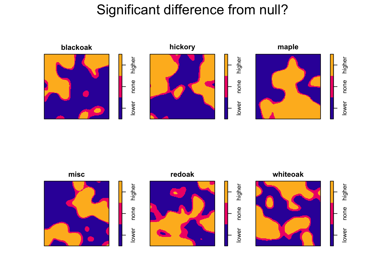
The final plot identifies where the spatially-varying probabilities exceed the null expected probability of each type. Areas of higher-than-expected probability could be considered “hot-spots” and areas of lower-than-expected probability could be considered “cold-spots.” Areas that are not significantly different from the null expectation could suggest additional sampling is necessary to determine if these areas are hot or cold spots.

Ian Buller, PhD, MA, GISP
Senior Epidemiologist
I am a (geo)spatial statistician & environmental epidemiologist who primarily codes in R • All content is my own and does not represent my employer • he/him/his