Plotting a Neighborhood Network with ggplot2
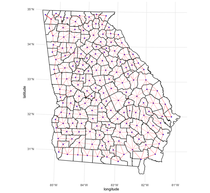 Image credit:
Ian Buller
Image credit:
Ian Buller
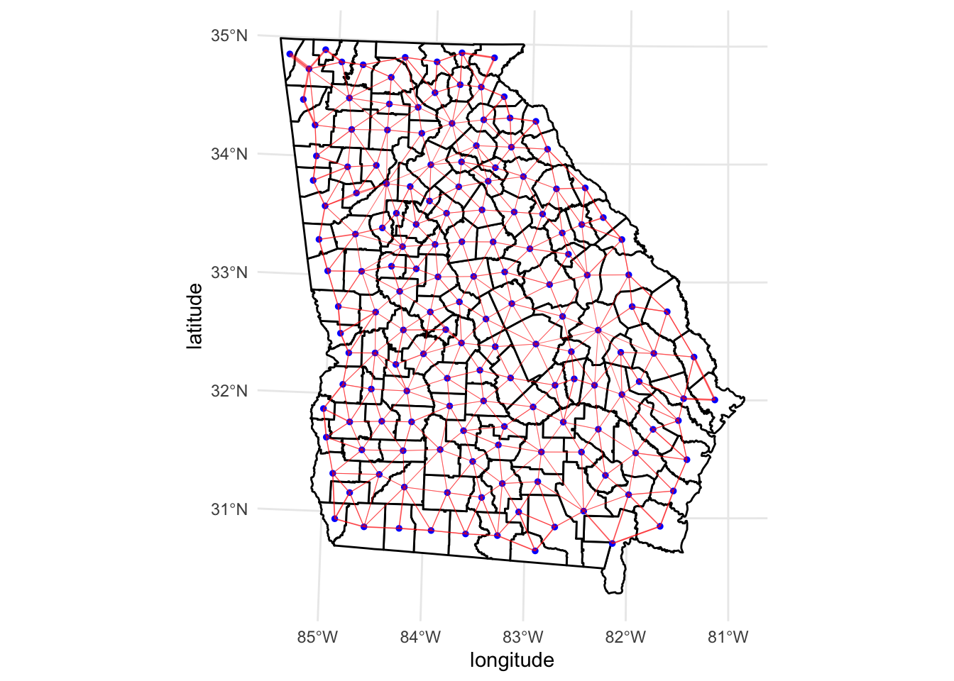
Here is an example of plotting a neighborhoods network with ggplot2 using the sf and sfdep packages for counties in a U.S. state.
We can display the “weights” feature of the neighborhoods network as the size of the line segments by scaling the size aesthetic with + scale_size_identity().
# Packages
loadedPackages <- c("ggplot2", "sf", "sfdep", "tigris")
invisible(lapply(loadedPackages, require, character.only = TRUE))

# County geometries of Georgia, U.S.A.
shp_ga <- counties(state = "Georgia", cb = TRUE)

# NAD83/UTM zone 17N geospatial projection
proj_ga <- st_transform(shp_ga, crs = 26917)

# First order contiguity (Queen's case by default)
nb <- st_contiguity(st_geometry(proj_ga))

# Contiguity-based spatial weights matrix
nbw <- st_weights(nb)

# County centroids
centroids <- st_centroid(proj_ga)

# Assign latitude and longitude for centroid connections in a dataframe
da <- data.frame(
  from = rep(1:length(nbw), attributes(nbw)$comp$d),
  to = unlist(nb),
  weight = unlist(nbw)
)
da <- cbind(
  da,
  st_coordinates(centroids)[da$from, 1:2],
  st_coordinates(centroids)[da$to, 1:2]
)
colnames(da)[4:7] <- c("longitude", "latitude", "long_to", "lat_to")
Plot counties and first order contiguity line segments with size scaled by “weights” feature.
ggplot() +
  geom_sf(data = proj_ga, fill = "white", color = "black") +
  geom_sf(data = centroids, color = "blue", size = 1) +
  geom_segment(
    data = da,
    aes(
      x = longitude,
      y = latitude,
      xend = long_to,
      yend = lat_to,
      size = weight
    ),
    color = "red",
    alpha = 0.5
  ) +
  scale_size_identity() +
  theme_minimal()
This answer was also posted to Stack Overflow. Some code modified from code by @ StupidWolf’s answer.
Ian Buller, PhD, MA
Epidemiologist
I am a (geo)spatial statistician & environmental epidemiologist who primarily codes in R • All content is my own and does not represent my employer • he/him/his